Hierarchical ITS for staggered launches (event-study)

This notebook demonstrates HierarchicalInterruptedTimeSeries, a multi-unit ITS design where each unit (e.g. a product) has its own treatment time. Per-unit intercepts, time trends, covariate slopes and the launch “lift” are partially pooled toward shared population-level hyperparameters, so sparse units borrow strength from well-observed ones and we recover a posterior over the population effect that can be used to forecast the impact of a new launch.

The model always includes hierarchical (random) linear time trends per unit, \(\gamma_i \sim \mathcal{N}(\mu_\gamma, \sigma_\gamma)\), so that the baseline for each unit can drift over time rather than being a flat intercept. This is important for avoiding confounding between secular trends and the treatment effect.

Four effect parameterizations are available:

• effect_type='instant' — a single post-launch level shift per unit.

• effect_type='saturation' — a Hill (logistic-type) saturation curve: the effect ramps up smoothly after launch and asymptotes at a per-unit ceiling, rather than jumping instantly to its final size.

• effect_type='event_study' — dynamic effects across post-launch event-time bins.

• effect_type='placebo' — the event-study form extended with pre-launch leads as placebos.

import matplotlib.pyplot as plt
import numpy as np
import pandas as pd
import pymc as pm

import causalpy as cp
from causalpy.pymc_models import HierarchicalLaunchITS

rng = np.random.default_rng(42)

Shared simulation utilities

Each of the three model variants is designed to handle a different kind of treatment effect, so in the sections below we simulate a different panel for each one to show how faithfully it recovers the truth. The helpers below build a panel of N_PRODUCTS products observed weekly over T weeks with per-product intercepts, covariate slopes, shared seasonality, and a user-supplied effect function effect_fn(tau) that returns the true causal contribution for a given event time tau = week - launch_week.

N_PRODUCTS = 15
T = 200


def fourier_terms(t, period=52, K=2):
    cols = []
    for k in range(1, K + 1):
        cols.append(np.sin(2 * np.pi * k * t / period))
        cols.append(np.cos(2 * np.pi * k * t / period))
    return np.column_stack(cols)


def simulate_panel(effect_fn, seed, n_products=N_PRODUCTS, T=T):
    """Simulate a staggered-launch panel with a user-supplied effect function.

    ``effect_fn(tau, i)`` receives event time (weeks since launch) and the
    product index and returns the true causal contribution to sales.

    Each unit has its own linear time trend ``trend_i ~ N(0.01, 0.005)`` —
    small enough that the staggered design can separate it from the treatment
    effect, but large enough to exercise the model's time-trend component.
    """
    rng = np.random.default_rng(seed)
    alpha = rng.normal(50, 8, n_products)
    trend = rng.normal(0.01, 0.005, n_products)  # per-unit time trend
    gamma = rng.normal(0.15, 0.03, n_products)
    delta = rng.normal(-0.6, 0.1, n_products)
    launch_week = rng.integers(40, T - 80, n_products)

    week_idx = np.arange(T)
    season = fourier_terms(week_idx) @ np.array([6.0, -3.0, 2.0, -1.5])

    rows = []
    for i in range(n_products):
        emails = rng.normal(120, 25, T)
        price = rng.normal(20, 2, T)
        tau = week_idx - launch_week[i]
        effect = effect_fn(tau, i, rng)
        sales = (
            alpha[i]
            + trend[i] * week_idx  # linear time trend per unit
            + gamma[i] * emails
            + delta[i] * price
            + season
            + effect
            + rng.normal(0, 4, T)
        )
        rows.append(
            pd.DataFrame(
                {
                    "product": i,
                    "week_idx": week_idx,
                    "launch_week": launch_week[i],
                    "sales": sales,
                    "emails": emails,
                    "price": price,
                }
            )
        )
    return pd.concat(rows, ignore_index=True)

Instant lift model

DGP: a flat post-launch step of size lift_i ~ N(12, 4). Each product’s effect is constant from the launch week onwards — the simplest causal story and the one the instant model is designed for.

TRUE_MU_LIFT = 12.0
TRUE_SIGMA_LIFT = 4.0
_lift_rng = np.random.default_rng(7)
_lift_i = _lift_rng.normal(TRUE_MU_LIFT, TRUE_SIGMA_LIFT, N_PRODUCTS)


def instant_effect(tau, i, rng):
    return _lift_i[i] * (tau >= 0).astype(float)


df_instant = simulate_panel(instant_effect, seed=0)

result_instant = cp.HierarchicalInterruptedTimeSeries(
    data=df_instant,
    formula="sales ~ 0 + emails + price",
    unit_col="product",
    time_col="week_idx",
    treatment_time_col="launch_week",
    effect_type="instant",
    seasonality={"period": 52, "K": 2},
    model=HierarchicalLaunchITS(
        sample_kwargs={
            "draws": 1000,
            "tune": 1500,
            "chains": 4,
            "target_accept": 0.95,
            "random_seed": 42,
            "progressbar": False,
        }
    ),
)
result_instant.summary()
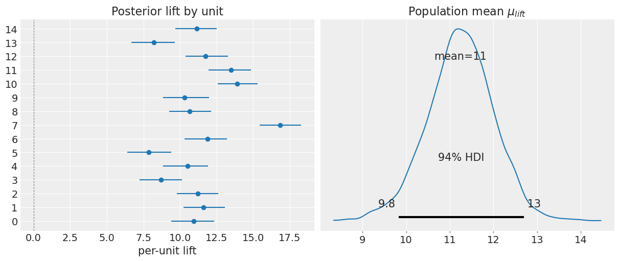
result_instant.plot();

Initializing NUTS using jitter+adapt_diag...
Multiprocess sampling (4 chains in 4 jobs)
NUTS: [mu_alpha, sigma_alpha, z_alpha, mu_gamma, sigma_gamma, z_gamma, mu_beta, sigma_beta, z_beta, beta_season, mu_lift, sigma_lift, z_lift, sigma]
/Users/nathanielforde/mambaforge/envs/CausalPy/lib/python3.14/site-packages/pymc/step_methods/hmc/quadpotential.py:316: RuntimeWarning: overflow encountered in dot
  return 0.5 * np.dot(x, v_out)
Sampling 4 chains for 1_500 tune and 1_000 draw iterations (6_000 + 4_000 draws total) took 128 seconds.
The rhat statistic is larger than 1.01 for some parameters. This indicates problems during sampling. See https://arxiv.org/abs/1903.08008 for details
The effective sample size per chain is smaller than 100 for some parameters.  A higher number is needed for reliable rhat and ess computation. See https://arxiv.org/abs/1903.08008 for details
Sampling: [beta_season, mu_alpha, mu_beta, mu_gamma, mu_lift, sigma, sigma_alpha, sigma_beta, sigma_gamma, sigma_lift, y_hat, z_alpha, z_beta, z_gamma, z_lift]
Sampling: [y_hat]
Sampling: [y_hat]
Sampling: [y_hat]

Hierarchical ITS (launch / event-study)
Formula: sales ~ 0 + emails + price
Effect type: instant
Units: 15
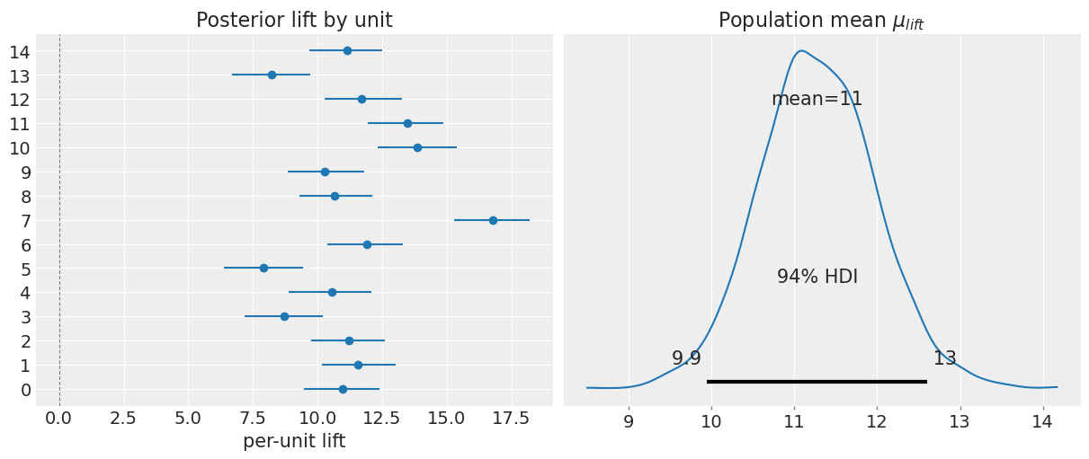
E[mu_lift] = 11.2   E[sigma_lift] = 2.61

Inspecting the fitted model

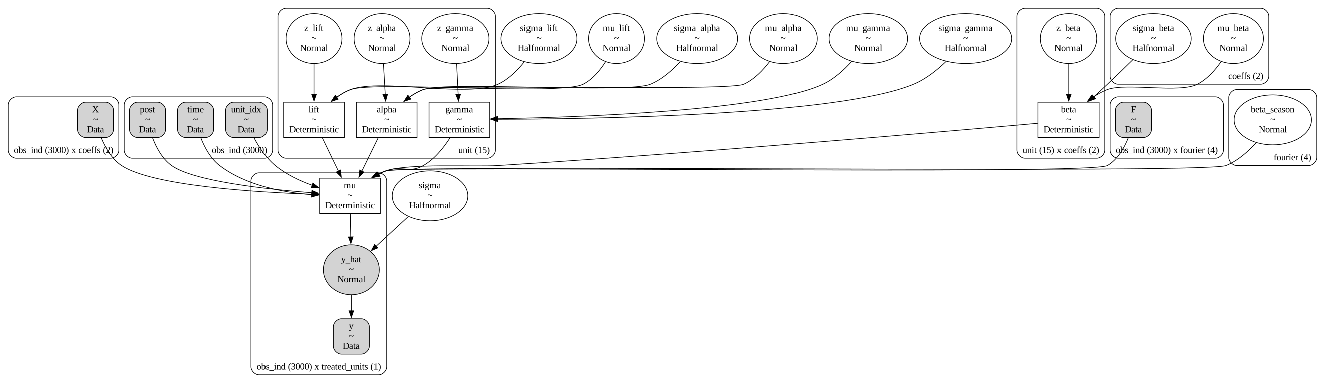
Every fitted HierarchicalInterruptedTimeSeries exposes the full PyMC posterior via result.idata (an ArviZ InferenceData object). From here you can visualise the model graph, check convergence, extract effect summaries, and compute Bayesian R².

# The model DAG — shows all hierarchical parameters and their dependencies
pm.model_to_graphviz(result_instant.model)

import arviz as az

# Convergence diagnostics for key hyperparameters: R-hat near 1.0 and
# large ESS (effective sample size) indicate healthy sampling.
az.summary(
    result_instant.idata,
    var_names=["mu_lift", "sigma_lift", "mu_gamma", "sigma_gamma", "sigma"],
)

	mean	sd	hdi_3%	hdi_97%	mcse_mean	mcse_sd	ess_bulk	ess_tail	r_hat
mu_lift	11.240	0.766	9.831	12.698	0.028	0.017	776.0	1410.0	1.0
sigma_lift	2.612	0.584	1.623	3.670	0.017	0.014	1201.0	2026.0	1.0
mu_gamma	0.734	0.166	0.437	1.064	0.003	0.003	2949.0	2338.0	1.0
sigma_gamma	0.313	0.195	0.001	0.632	0.007	0.003	767.0	1001.0	1.0
sigma	3.974	0.052	3.882	4.073	0.001	0.001	6222.0	2970.0	1.0

# effect_summary() returns an EffectSummary with a .table (DataFrame) and
# .text (prose). The table reports posterior mean, HDI, and the probability
# that the effect is positive — a quick decision-making summary.
es = result_instant.effect_summary()
display(es.table)
print(es.text)

	mean	hdi_95_low	hdi_95_high	prob_positive
parameter
mu_lift	11.240289	9.649514	12.674919	1.0
sigma_lift	2.612079	1.709416	3.972569	1.0

Post-period: Hierarchical ITS (launch / event-study)
Effect type: instant
Units: 15

# Bayesian R² — how much variance in the outcome is explained by the model.
result_instant.score

unit_0_r2        0.892759
unit_0_r2_std    0.001286
dtype: float64

Predictive distribution for a new launch

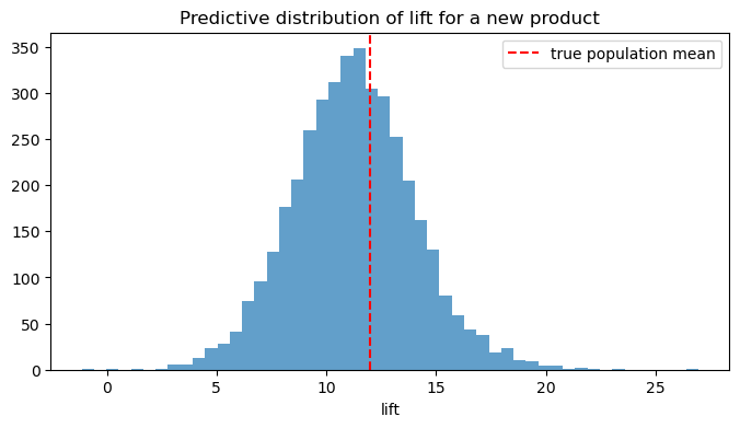
Because the model has a posterior over the population hyperparameters, we can sample the lift we would expect from a yet-unobserved product.

new_lift = result_instant.predictive_for_new_unit(size=4000, random_seed=0)
fig, ax = plt.subplots(figsize=(8, 4))
ax.hist(new_lift, bins=50, alpha=0.7)
ax.axvline(TRUE_MU_LIFT, color="red", ls="--", label="true population mean")
ax.set_title("Predictive distribution of lift for a new product")
ax.set_xlabel("lift")
ax.legend()
plt.show()

Observed vs counterfactual (single unit)

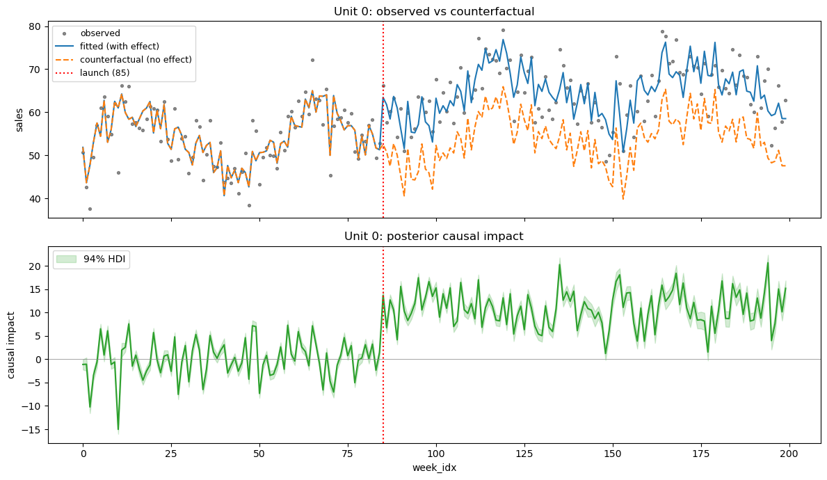
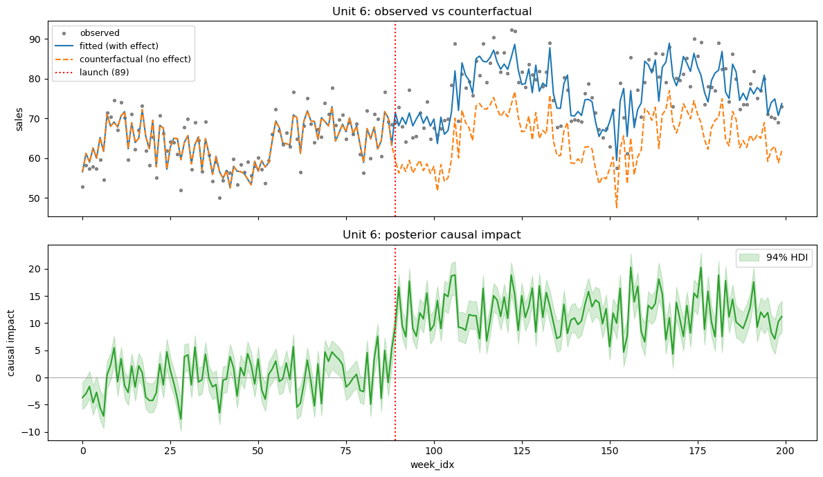
The fitted experiment stores three key objects for causal reasoning:

• result.observed_pred — posterior predictive under the actual design (with treatment effect switched on).

• result.counterfactual_pred — posterior predictive under the counterfactual design (treatment effect zeroed out — what would have happened without launch).

• result.impact — observed - counterfactual, the unit-level posterior of the causal effect at every time point.

The plot_unit() method visualises all three for a single product.

result_instant.plot_unit(unit_id=0)
plt.show()

Saturation (Hill-curve) model

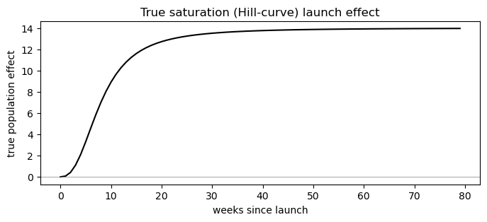
DGP: rather than an instant step, the true effect follows a Hill (logistic-type) saturation curve in event time — it ramps up smoothly after launch and asymptotes at a per-unit ceiling L_i, reaching half of that ceiling after k_i weeks:

\[ \text{effect}_i(\tau) = L_i \cdot \frac{\tau^s}{k_i^s + \tau^s}, \qquad \tau = \text{week} - \text{launch\_week} \ge 0 \]

This is the same functional form used for diminishing-returns / adstock saturation in media-mix models — here the “dose” is simply time-since-launch. It’s a much closer description of how adoption, distribution build and awareness actually accumulate after a real launch than an instant jump. effect_type='saturation' fits L_i and k_i hierarchically per unit (log scale, non-centered); the Hill exponent s (curve sharpness) is a single shared population parameter.

def hill(x, k, s):
    """Hill (logistic-type) saturation curve, x clipped to [0, inf)."""
    x = np.clip(np.asarray(x, dtype=float), 0, None)
    return x**s / (k**s + x**s)


TRUE_L_MEAN = 14.0  # ceiling lift, population mean
TRUE_L_SD_LOG = 0.15  # per-unit heterogeneity (log scale)
TRUE_K_MEAN = 8.0  # half-saturation time (weeks), population mean
TRUE_K_SD_LOG = 0.15
TRUE_S = 2.5  # Hill exponent (shared across units)

_sat_rng = np.random.default_rng(13)
_L_i = np.exp(_sat_rng.normal(np.log(TRUE_L_MEAN), TRUE_L_SD_LOG, N_PRODUCTS))
_k_i = np.exp(_sat_rng.normal(np.log(TRUE_K_MEAN), TRUE_K_SD_LOG, N_PRODUCTS))


def saturation_effect(tau, i, rng):
    return _L_i[i] * hill(tau, _k_i[i], TRUE_S)


df_saturation = simulate_panel(saturation_effect, seed=3)

# Show the true population saturation curve we expect to recover.
tau_grid = np.arange(0, 80)
fig, ax = plt.subplots(figsize=(8, 3))
ax.plot(tau_grid, TRUE_L_MEAN * hill(tau_grid, TRUE_K_MEAN, TRUE_S), color="black")
ax.axhline(0, color="grey", lw=0.5)
ax.set_xlabel("weeks since launch")
ax.set_ylabel("true population effect")
ax.set_title("True saturation (Hill-curve) launch effect")
plt.show()

result_saturation = cp.HierarchicalInterruptedTimeSeries(
    data=df_saturation,
    formula="sales ~ 0 + emails + price",
    unit_col="product",
    time_col="week_idx",
    treatment_time_col="launch_week",
    effect_type="saturation",
    seasonality={"period": 52, "K": 2},
    model=HierarchicalLaunchITS(
        sample_kwargs={
            "draws": 1000,
            "tune": 1500,
            "chains": 4,
            "target_accept": 0.95,
            "random_seed": 42,
            "progressbar": False,
        }
    ),
)
result_saturation.summary()
result_saturation.plot();

Initializing NUTS using jitter+adapt_diag...
Multiprocess sampling (4 chains in 4 jobs)
NUTS: [mu_alpha, sigma_alpha, z_alpha, mu_gamma, sigma_gamma, z_gamma, mu_beta, sigma_beta, z_beta, beta_season, mu_logL, sigma_logL, z_logL, mu_logk, sigma_logk, z_logk, s, sigma]
/Users/nathanielforde/mambaforge/envs/CausalPy/lib/python3.14/site-packages/pymc/step_methods/hmc/quadpotential.py:316: RuntimeWarning: overflow encountered in dot
  return 0.5 * np.dot(x, v_out)
Sampling 4 chains for 1_500 tune and 1_000 draw iterations (6_000 + 4_000 draws total) took 327 seconds.
The rhat statistic is larger than 1.01 for some parameters. This indicates problems during sampling. See https://arxiv.org/abs/1903.08008 for details
The effective sample size per chain is smaller than 100 for some parameters.  A higher number is needed for reliable rhat and ess computation. See https://arxiv.org/abs/1903.08008 for details
Sampling: [beta_season, mu_alpha, mu_beta, mu_gamma, mu_logL, mu_logk, s, sigma, sigma_alpha, sigma_beta, sigma_gamma, sigma_logL, sigma_logk, y_hat, z_alpha, z_beta, z_gamma, z_logL, z_logk]
Sampling: [y_hat]
Sampling: [y_hat]
Sampling: [y_hat]

Hierarchical ITS (launch / event-study)
Formula: sales ~ 0 + emails + price
Effect type: saturation
Units: 15
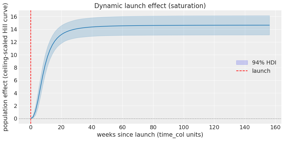
E[L] (ceiling lift) = 14.7   E[k] (half-saturation time) = 8.43   E[s] (Hill exponent) = 2.55

/Users/nathanielforde/Documents/Github/CausalPy/causalpy/experiments/hierarchical_interrupted_time_series.py:621: UserWarning: The figure layout has changed to tight
  fig.tight_layout()

Convergence diagnostics and effect summary

L and k are fit hierarchically on the log scale (mu_logL/sigma_logL, mu_logk/sigma_logk); s is a single shared parameter. effect_summary() reports the population-level ceiling lift, half-saturation time and Hill exponent on their natural (exponentiated) scale.

# R-hat near 1.0 and large ESS indicate healthy sampling.
display(
    az.summary(
        result_saturation.idata,
        var_names=[
            "mu_logL",
            "sigma_logL",
            "mu_logk",
            "sigma_logk",
            "s",
            "mu_gamma",
            "sigma_gamma",
            "sigma",
        ],
    )
)

es = result_saturation.effect_summary()
display(es.table)
print(es.text)

	mean	sd	hdi_3%	hdi_97%	mcse_mean	mcse_sd	ess_bulk	ess_tail	r_hat
mu_logL	2.683	0.056	2.573	2.780	0.002	0.001	1190.0	2143.0	1.0
sigma_logL	0.177	0.046	0.097	0.260	0.001	0.001	1535.0	1918.0	1.0
mu_logk	2.129	0.077	1.982	2.270	0.001	0.001	2859.0	3028.0	1.0
sigma_logk	0.233	0.074	0.100	0.365	0.002	0.001	1577.0	2572.0	1.0
s	2.553	0.269	2.061	3.078	0.004	0.004	5773.0	3226.0	1.0
mu_gamma	0.634	0.210	0.252	1.045	0.003	0.003	3850.0	3084.0	1.0
sigma_gamma	0.302	0.211	0.000	0.677	0.006	0.004	1026.0	1676.0	1.0
sigma	4.099	0.054	3.997	4.200	0.001	0.001	8317.0	2920.0	1.0

	mean	hdi_95_low	hdi_95_high	prob_positive
parameter
L (ceiling lift)	14.650835	13.077124	16.244950	1.0
k (half-saturation time)	8.433520	7.217934	9.774802	1.0
s (Hill exponent)	2.553101	2.071411	3.148848	1.0

Post-period: Hierarchical ITS (launch / event-study)
Effect type: saturation
Units: 15

Population predictive curve for a new unit

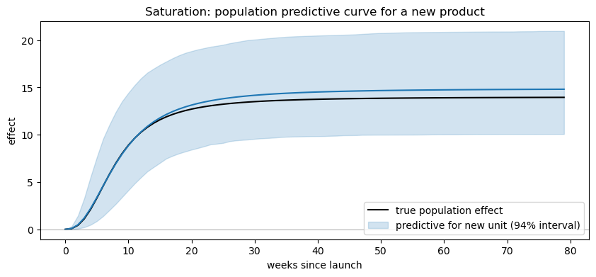
For effect_type='saturation', predictive_for_new_unit returns a (draws, 3) array of [L, k, s] samples for a hypothetical new product. Turning each draw into a full Hill curve and overlaying the resulting predictive band on the true population curve shows how well the model recovers both how big (L) and how fast (k) the effect is.

new_sat = result_saturation.predictive_for_new_unit(size=4000, random_seed=0)
# new_sat shape: (4000, 3) -> columns [L, k, s]
tau_grid = np.arange(0, 80)
L_draws, k_draws, s_draws = new_sat[:, 0], new_sat[:, 1], new_sat[:, 2]
curves = L_draws[:, None] * hill(tau_grid[None, :], k_draws[:, None], s_draws[:, None])
pred_mean = curves.mean(axis=0)
pred_lo = np.percentile(curves, 3, axis=0)
pred_hi = np.percentile(curves, 97, axis=0)

fig, ax = plt.subplots(figsize=(10, 4))
ax.plot(
    tau_grid,
    TRUE_L_MEAN * hill(tau_grid, TRUE_K_MEAN, TRUE_S),
    color="black",
    label="true population effect",
)
ax.fill_between(
    tau_grid,
    pred_lo,
    pred_hi,
    color="C0",
    alpha=0.2,
    label="predictive for new unit (94% interval)",
)
ax.plot(tau_grid, pred_mean, color="C0")
ax.axhline(0, color="grey", lw=0.5)
ax.set_xlabel("weeks since launch")
ax.set_ylabel("effect")
ax.set_title("Saturation: population predictive curve for a new product")
ax.legend()
plt.show()

Observed vs counterfactual (single unit)

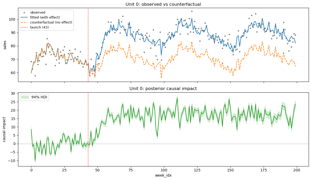
Same three objects as the instant model (observed_pred, counterfactual_pred, impact) — but now the counterfactual gap traces out the shape of the Hill curve, ramping up after launch, rather than jumping instantly to a constant lift.

result_saturation.plot_unit(unit_id=0)
plt.show()

Event-study (dynamic) model

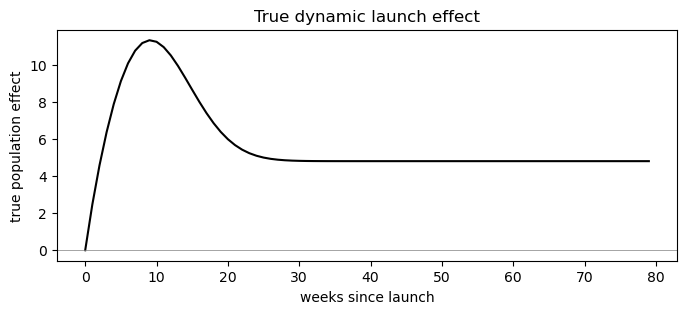
DGP: a realistic launch curve — awareness ramps up over the first few weeks, peaks around week 8, then decays toward a lower long-run level as novelty wears off. A single “instant” lift would average this over time and miss the story entirely; the event-study variant estimates a separate population effect per post-launch bin and should trace out the true curve.

TRUE_MU_AMP = 12.0
TRUE_SIGMA_AMP = 3.0
_amp_rng = np.random.default_rng(11)
_amp_i = _amp_rng.normal(TRUE_MU_AMP, TRUE_SIGMA_AMP, N_PRODUCTS)


def launch_shape(tau):
    """Ramp-up, peak around week 8, decay toward ~40% long-run level."""
    tau = np.asarray(tau, dtype=float)
    return np.where(
        tau < 0,
        0.0,
        (1 - np.exp(-tau / 3.0)) * (0.4 + 0.6 * np.exp(-((tau - 8.0) ** 2) / 80.0)),
    )


def dynamic_effect(tau, i, rng):
    return _amp_i[i] * launch_shape(tau)


df_event = simulate_panel(dynamic_effect, seed=1)

# Show the true population event-time curve we expect to recover.
tau_grid = np.arange(0, 80)
fig, ax = plt.subplots(figsize=(8, 3))
ax.plot(tau_grid, TRUE_MU_AMP * launch_shape(tau_grid), color="black")
ax.axhline(0, color="grey", lw=0.5)
ax.set_xlabel("weeks since launch")
ax.set_ylabel("true population effect")
ax.set_title("True dynamic launch effect")
plt.show()

result_event = cp.HierarchicalInterruptedTimeSeries(
    data=df_event,
    formula="sales ~ 0 + emails + price",
    unit_col="product",
    time_col="week_idx",
    treatment_time_col="launch_week",
    effect_type="event_study",
    bin_edges=[0, 4, 8, 12, 16, 20, 26, 39, 52, 78, 10000],
    seasonality={"period": 52, "K": 2},
    model=HierarchicalLaunchITS(
        sample_kwargs={
            "draws": 1000,
            "tune": 1500,
            "chains": 4,
            "target_accept": 0.95,
            "random_seed": 42,
            "progressbar": False,
        }
    ),
)
result_event.summary()
result_event.plot();

Initializing NUTS using jitter+adapt_diag...
Multiprocess sampling (4 chains in 4 jobs)
NUTS: [mu_alpha, sigma_alpha, z_alpha, mu_gamma, sigma_gamma, z_gamma, mu_beta, sigma_beta, z_beta, beta_season, mu_delta, sigma_delta, z_delta, sigma]
/Users/nathanielforde/mambaforge/envs/CausalPy/lib/python3.14/site-packages/pymc/step_methods/hmc/quadpotential.py:316: RuntimeWarning: overflow encountered in dot
  return 0.5 * np.dot(x, v_out)
Sampling 4 chains for 1_500 tune and 1_000 draw iterations (6_000 + 4_000 draws total) took 221 seconds.
Sampling: [beta_season, mu_alpha, mu_beta, mu_delta, mu_gamma, sigma, sigma_alpha, sigma_beta, sigma_delta, sigma_gamma, y_hat, z_alpha, z_beta, z_delta, z_gamma]
Sampling: [y_hat]
Sampling: [y_hat]
Sampling: [y_hat]

Hierarchical ITS (launch / event-study)
Formula: sales ~ 0 + emails + price
Effect type: event_study
Units: 15
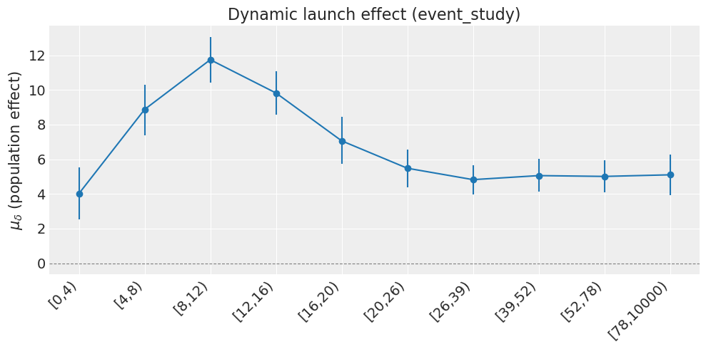
  [0,4)               mu_delta = +4.02
  [4,8)               mu_delta = +8.87
  [8,12)              mu_delta = +11.7
  [12,16)             mu_delta = +9.82
  [16,20)             mu_delta = +7.06
  [20,26)             mu_delta = +5.48
  [26,39)             mu_delta = +4.82
  [39,52)             mu_delta = +5.05
  [52,78)             mu_delta = +5.01
  [78,10000)          mu_delta = +5.1

/Users/nathanielforde/Documents/Github/CausalPy/causalpy/experiments/hierarchical_interrupted_time_series.py:668: UserWarning: The figure layout has changed to tight
  fig.tight_layout()

Population predictive for a new unit

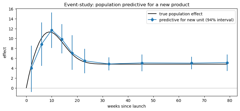
For the event-study variant, predictive_for_new_unit returns a (draws, n_bins) array — one draw from \(\mathcal{N}(\mu_\delta, \sigma_\delta)\) per bin per posterior sample. We can overlay the posterior mean and HDI on the true population curve to see how well the model recovers the dynamic launch shape.

new_delta = result_event.predictive_for_new_unit(size=4000, random_seed=0)
# new_delta shape: (4000, n_bins)
bin_edges = [0, 4, 8, 12, 16, 20, 26, 39, 52, 78, 10000]
bin_mids = [
    0.5 * (bin_edges[k] + min(bin_edges[k + 1], 80)) for k in range(len(bin_edges) - 1)
]

fig, ax = plt.subplots(figsize=(10, 4))
# True curve
tau_grid = np.arange(0, 80)
ax.plot(
    tau_grid,
    TRUE_MU_AMP * launch_shape(tau_grid),
    color="black",
    label="true population effect",
)
# Posterior predictive for new unit
pred_mean = new_delta.mean(axis=0)
pred_lo = np.percentile(new_delta, 3, axis=0)
pred_hi = np.percentile(new_delta, 97, axis=0)
ax.errorbar(
    bin_mids,
    pred_mean,
    yerr=np.vstack([pred_mean - pred_lo, pred_hi - pred_mean]),
    fmt="o-",
    color="C0",
    label="predictive for new unit (94% interval)",
)
ax.axhline(0, color="grey", lw=0.5)
ax.set_xlabel("weeks since launch")
ax.set_ylabel("effect")
ax.set_title("Event-study: population predictive for a new product")
ax.legend()
plt.show()

Placebo (lead/lag) model

DGP: we generate two panels from the same random seed (so the noise, covariates and launch weeks are identical) but with different treatment effects:

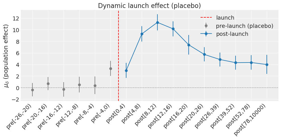
1. With anticipation — the ramp/peak/decay post-launch curve plus a deliberate pre-launch linear build-up over the 8 weeks before launch (e.g. a pre-order period). The placebo bins in [-8, -4) and [-4, 0) should absorb this and the automatic check should fail.

2. Without anticipation — the same post-launch dynamics but strictly zero before launch. The placebo bins should be indistinguishable from zero and the check should pass.

Because the only difference between the two panels is the anticipation component, the contrast isolates exactly what the placebo test is designed to detect.

def anticipation_effect(tau, i, rng):
    """Dynamic post-launch effect + pre-launch build-up over 8 weeks."""
    post = _amp_i[i] * launch_shape(tau)
    tau_arr = np.asarray(tau, dtype=float)
    lead = np.where(
        (tau_arr >= -8) & (tau_arr < 0),
        _amp_i[i] * 0.4 * (tau_arr + 8) / 8.0,  # linear ramp up to ~40% of amp
        0.0,
    )
    return post + lead


def clean_dynamic_effect(tau, i, rng):
    """Same post-launch dynamics, but strictly zero before launch."""
    return _amp_i[i] * launch_shape(tau)


# Same seed → identical noise; only difference is the anticipation component
df_placebo_bad = simulate_panel(anticipation_effect, seed=2)
df_placebo_clean = simulate_panel(clean_dynamic_effect, seed=2)


def make_placebo_model():
    return HierarchicalLaunchITS(
        sample_kwargs={
            "draws": 1000,
            "tune": 1500,
            "chains": 4,
            "target_accept": 0.97,
            "random_seed": 42,
            "progressbar": False,
        }
    )


placebo_kwargs = {
    "formula": "sales ~ 0 + emails + price",
    "unit_col": "product",
    "time_col": "week_idx",
    "treatment_time_col": "launch_week",
    "effect_type": "placebo",
    "bin_edges": [0, 4, 8, 12, 16, 20, 26, 39, 52, 78, 10000],
    "placebo_edges": [-26, -20, -16, -12, -8, -4, 0],
    "seasonality": {"period": 52, "K": 2},
}

print("=== Panel WITH anticipation (placebo check should FAIL) ===")
result_placebo_bad = cp.HierarchicalInterruptedTimeSeries(
    data=df_placebo_bad, model=make_placebo_model(), **placebo_kwargs
)
result_placebo_bad.summary()
result_placebo_bad.plot();

=== Panel WITH anticipation (placebo check should FAIL) ===

Initializing NUTS using jitter+adapt_diag...
Multiprocess sampling (4 chains in 4 jobs)
NUTS: [mu_alpha, sigma_alpha, z_alpha, mu_gamma, sigma_gamma, z_gamma, mu_beta, sigma_beta, z_beta, beta_season, mu_delta, sigma_delta, z_delta, sigma]
Sampling 4 chains for 1_500 tune and 1_000 draw iterations (6_000 + 4_000 draws total) took 573 seconds.
The rhat statistic is larger than 1.01 for some parameters. This indicates problems during sampling. See https://arxiv.org/abs/1903.08008 for details
Sampling: [beta_season, mu_alpha, mu_beta, mu_delta, mu_gamma, sigma, sigma_alpha, sigma_beta, sigma_delta, sigma_gamma, y_hat, z_alpha, z_beta, z_delta, z_gamma]
Sampling: [y_hat]
Sampling: [y_hat]
Sampling: [y_hat]

Hierarchical ITS (launch / event-study)
Formula: sales ~ 0 + emails + price
Effect type: placebo
Units: 15
  pre[-26,-20)        mu_delta = -0.364
  pre[-20,-16)        mu_delta = +0.684
  pre[-16,-12)        mu_delta = -0.296
  pre[-12,-8)         mu_delta = +0.515
  pre[-8,-4)          mu_delta = +0.365
  pre[-4,0)           mu_delta = +3.32
  post[0,4)           mu_delta = +2.96
  post[4,8)           mu_delta = +9.27
  post[8,12)          mu_delta = +11.3
  post[12,16)         mu_delta = +10.2
  post[16,20)         mu_delta = +7.4
  post[20,26)         mu_delta = +5.73
  post[26,39)         mu_delta = +4.85
  post[39,52)         mu_delta = +4.31
  post[52,78)         mu_delta = +4.34
  post[78,10000)      mu_delta = +3.99
Placebo check: FAIL (5/6 pre-launch bins contain 0 within the 94% HDI)

/Users/nathanielforde/Documents/Github/CausalPy/causalpy/experiments/hierarchical_interrupted_time_series.py:668: UserWarning: The figure layout has changed to tight
  fig.tight_layout()

print("=== Same noise, NO anticipation (placebo check should PASS) ===")
result_placebo_ok = cp.HierarchicalInterruptedTimeSeries(
    data=df_placebo_clean, model=make_placebo_model(), **placebo_kwargs
)
result_placebo_ok.summary()
result_placebo_ok.plot();

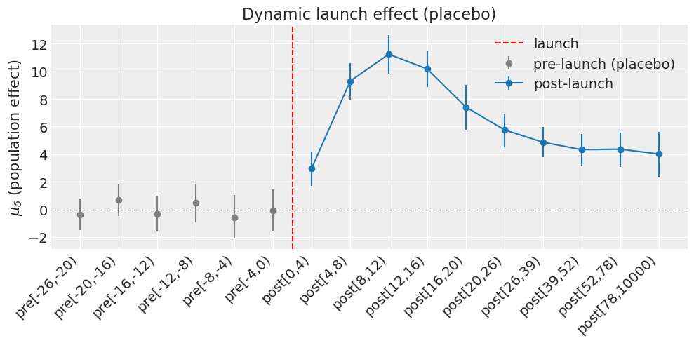
=== Same noise, NO anticipation (placebo check should PASS) ===

Initializing NUTS using jitter+adapt_diag...
Multiprocess sampling (4 chains in 4 jobs)
NUTS: [mu_alpha, sigma_alpha, z_alpha, mu_gamma, sigma_gamma, z_gamma, mu_beta, sigma_beta, z_beta, beta_season, mu_delta, sigma_delta, z_delta, sigma]
Sampling 4 chains for 1_500 tune and 1_000 draw iterations (6_000 + 4_000 draws total) took 600 seconds.
The effective sample size per chain is smaller than 100 for some parameters.  A higher number is needed for reliable rhat and ess computation. See https://arxiv.org/abs/1903.08008 for details
Sampling: [beta_season, mu_alpha, mu_beta, mu_delta, mu_gamma, sigma, sigma_alpha, sigma_beta, sigma_delta, sigma_gamma, y_hat, z_alpha, z_beta, z_delta, z_gamma]
Sampling: [y_hat]
Sampling: [y_hat]
Sampling: [y_hat]

Hierarchical ITS (launch / event-study)
Formula: sales ~ 0 + emails + price
Effect type: placebo
Units: 15
  pre[-26,-20)        mu_delta = -0.377
  pre[-20,-16)        mu_delta = +0.673
  pre[-16,-12)        mu_delta = -0.311
  pre[-12,-8)         mu_delta = +0.494
  pre[-8,-4)          mu_delta = -0.56
  pre[-4,0)           mu_delta = -0.0915
  post[0,4)           mu_delta = +2.97
  post[4,8)           mu_delta = +9.29
  post[8,12)          mu_delta = +11.2
  post[12,16)         mu_delta = +10.2
  post[16,20)         mu_delta = +7.41
  post[20,26)         mu_delta = +5.76
  post[26,39)         mu_delta = +4.86
  post[39,52)         mu_delta = +4.33
  post[52,78)         mu_delta = +4.36
  post[78,10000)      mu_delta = +4.02
Placebo check: PASS (6/6 pre-launch bins contain 0 within the 94% HDI)

/Users/nathanielforde/Documents/Github/CausalPy/causalpy/experiments/hierarchical_interrupted_time_series.py:668: UserWarning: The figure layout has changed to tight
  fig.tight_layout()

Model diagnostics

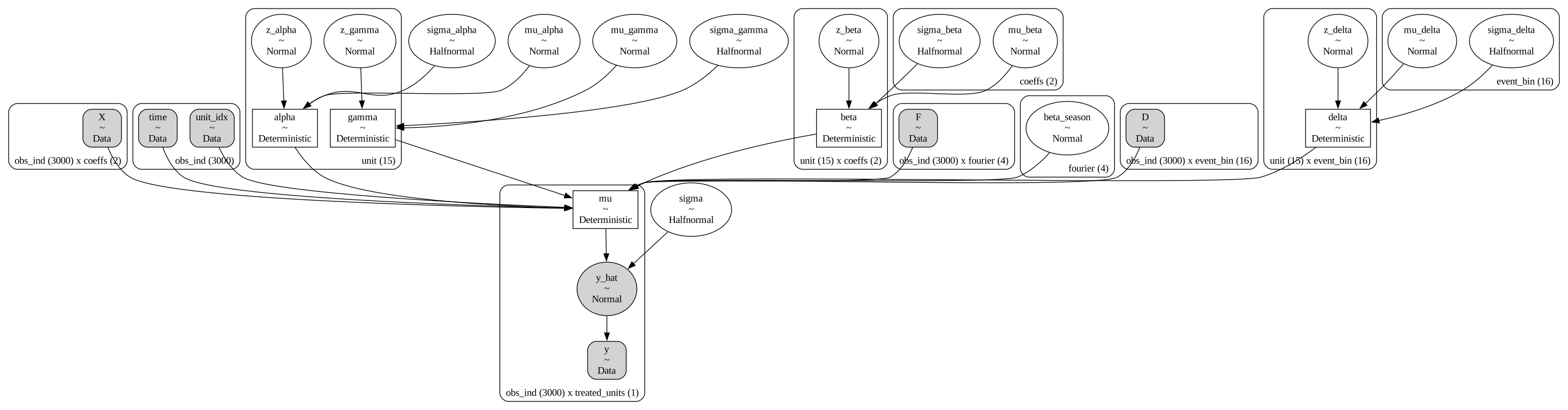
The underlying HierarchicalLaunchITS is a standard PyMC model, so we can use pm.model_to_graphviz to visualise the DAG, ArviZ trace plots to check convergence, and az.summary for R-hat / ESS diagnostics. These are essential sanity checks before trusting the causal estimates.

Model graph — the plate diagram shows the hierarchical structure: population hyperparameters at the top, per-unit parameters inside the “unit” plate, and the likelihood at the bottom.

pm.model_to_graphviz(result_placebo_ok.model)

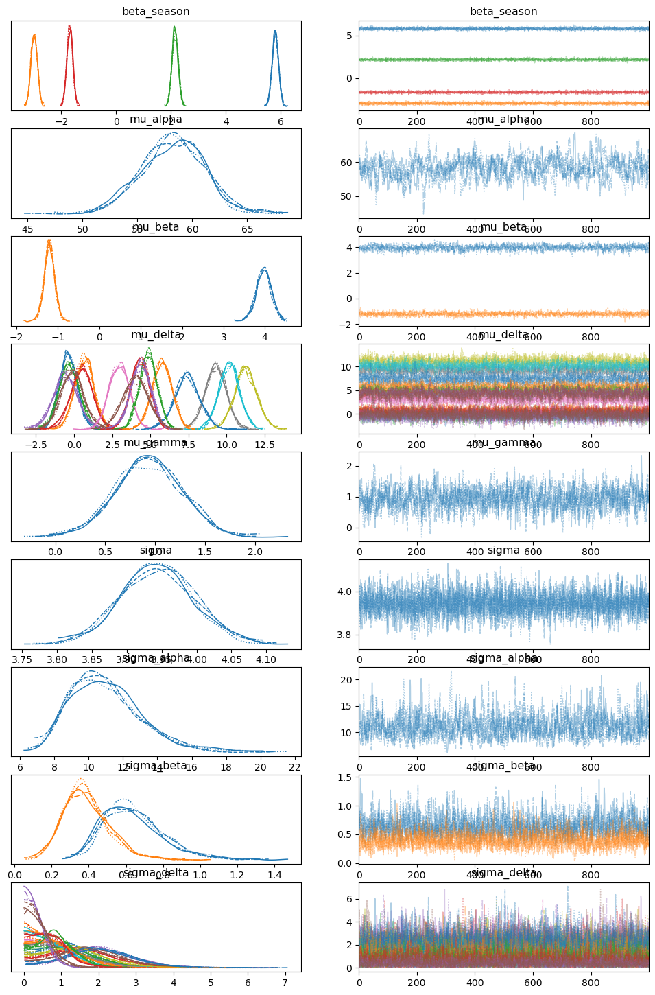
Trace plots — each row shows a population-level hyperparameter. Look for: chains that overlap and appear stationary (good mixing), no sustained trends, and no divergences flagged in the sampling output. The right-hand marginal posteriors should be smooth and unimodal.

import arviz as az

az.plot_trace(
    result_placebo_ok.idata,
    var_names=[
        "beta_season",
        "mu_alpha",
        "mu_beta",
        "mu_delta",
        "mu_gamma",
        "sigma",
        "sigma_alpha",
        "sigma_beta",
        "sigma_delta",
    ],
)
plt.show()

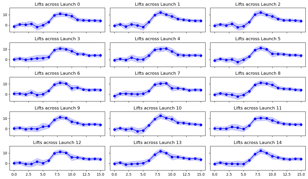
Per-unit effect profiles — each panel below shows one product’s posterior delta coefficients across the 16 event-time bins (6 pre-launch placebos + 10 post-launch).

fig, axs = plt.subplots(5, 3, figsize=(12, 7), sharex=True, sharey=True)
axs = axs.flatten()
summary_delta = az.summary(result_placebo_ok.idata, var_names=["delta"], hdi_prob=0.94)
summary_delta["index_col"] = summary_delta.index

summary_delta["index_col"] = summary_delta["index_col"].str.split("delta\[").str[1]
summary_delta["index_col"] = (
    summary_delta["index_col"].str.split(",").str[0].astype(int)
)
for i, ax in enumerate(axs):
    row = summary_delta[summary_delta["index_col"] == i]
    ax.plot(range(16), row["mean"], marker="o", ls="-", color="blue")
    ax.fill_between(range(16), row["hdi_3%"], row["hdi_97%"], color="blue", alpha=0.2)
    ax.set_title(f"Lifts across Launch {i}")
plt.tight_layout()

AR(1) residuals (optional)

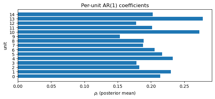
Time series residuals are rarely i.i.d. When autocorrelation is present, the default Normal noise can produce overconfident uncertainty intervals. Passing ar_residuals=True adds a hierarchical AR(1) process to the residuals, implemented via pytensor.scan:

\[ e_{i,t} = \rho_i \, e_{i,t-1} + \varepsilon_{i,t}, \qquad \rho_i \sim \tanh\!\bigl(\mathcal{N}(\mu_\rho, \sigma_\rho)\bigr) \]

The tanh link ensures stationarity (\(|\rho_i| < 1\)). This requires a balanced panel (all units observed at the same time steps).

result_ar = cp.HierarchicalInterruptedTimeSeries(
    data=df_instant,
    formula="sales ~ 0 + emails + price",
    unit_col="product",
    time_col="week_idx",
    treatment_time_col="launch_week",
    effect_type="instant",
    seasonality={"period": 52, "K": 2},
    ar_residuals=True,
    model=HierarchicalLaunchITS(
        sample_kwargs={
            "draws": 1000,
            "tune": 1500,
            "chains": 4,
            "target_accept": 0.95,
            "random_seed": 42,
            "progressbar": False,
        }
    ),
)
result_ar.summary()
result_ar.plot();

Initializing NUTS using jitter+adapt_diag...
Multiprocess sampling (4 chains in 4 jobs)
NUTS: [mu_alpha, sigma_alpha, z_alpha, mu_gamma, sigma_gamma, z_gamma, mu_beta, sigma_beta, z_beta, beta_season, mu_lift, sigma_lift, z_lift, mu_rho, sigma_rho, z_rho, z_ar, sigma_ar, sigma]
Sampling 4 chains for 1_500 tune and 1_000 draw iterations (6_000 + 4_000 draws total) took 377 seconds.
The rhat statistic is larger than 1.01 for some parameters. This indicates problems during sampling. See https://arxiv.org/abs/1903.08008 for details
The effective sample size per chain is smaller than 100 for some parameters.  A higher number is needed for reliable rhat and ess computation. See https://arxiv.org/abs/1903.08008 for details
Sampling: [beta_season, mu_alpha, mu_beta, mu_gamma, mu_lift, mu_rho, sigma, sigma_alpha, sigma_ar, sigma_beta, sigma_gamma, sigma_lift, sigma_rho, y_hat, z_alpha, z_ar, z_beta, z_gamma, z_lift, z_rho]
Sampling: [y_hat]
Sampling: [y_hat]
Sampling: [y_hat]

Hierarchical ITS (launch / event-study)
Formula: sales ~ 0 + emails + price
Effect type: instant
Units: 15
E[mu_lift] = 11.3   E[sigma_lift] = 2.61

post_ar = result_ar.model.idata.posterior
rho_mean = post_ar["rho"].mean(("chain", "draw")).values
fig, ax = plt.subplots(figsize=(8, 3))
ax.barh(range(len(rho_mean)), rho_mean)
ax.set_yticks(range(len(rho_mean)))
ax.set_xlabel(r"$\rho_i$ (posterior mean)")
ax.set_ylabel("unit")
ax.set_title("Per-unit AR(1) coefficients")
ax.axvline(0, color="grey", lw=0.5)
plt.show()

result_ar.plot_unit(unit_id=6)
plt.show()

Notes on the implementation

• All hierarchical parameters use a non-centered parametrization for sampler health.

• Hierarchical linear time trends \(\gamma_i \sim \mathcal{N}(\mu_\gamma, \sigma_\gamma)\) are always included, allowing each unit’s baseline to drift linearly over time. The time index is standardized internally for numerical stability.

• Saturation (effect_type='saturation') replaces the instant level shift with a Hill curve, \(\text{effect}_i(\tau) = L_i \, \tau^s / (k_i^s + \tau^s)\). The ceiling lift \(L_i\) and half-saturation time \(k_i\) are hierarchical per unit (log scale, non-centered); the Hill exponent \(s\) is a single shared population parameter. mu_logk/sigma_logk/s use fixed, generic priors (not data-adaptive to time_col’s scale) — override them via priors= if your time index isn’t in “a handful of periods to ramp up” units, e.g. daily rather than weekly data.

• Optional AR(1) residuals (ar_residuals=True) add per-unit autocorrelated noise via pytensor.scan. The AR coefficient is constrained to \((-1, 1)\) via a tanh link and partially pooled across units. Requires a balanced panel.

• Priors on population-level scale parameters are derived from the data via priors_from_data so the model is approximately scale-invariant.

• Covariates from the patsy formula are standardized internally; the hierarchical \(\alpha\) takes the place of an intercept (you should not include one in formula). print_coefficients() also reports covariate coefficients back on their original (unstandardized) scale.

• Any prior can be overridden via the priors= argument to HierarchicalLaunchITS using the pymc_extras.prior.Prior system.